
earthaccess and the cloud, the force awakens
Luis A. López
NSIDC, NASA Openscapes
NASA ESDS Tech Spotlight, Feb 2024
Art: Allison Horts
Notes:
Disclaimer: Opinions expressed here are solely my own and do not express the views or opinions of my employer.
This notebook runs out of a local experimental environment that has not been pushed to the main earthaccess repository and is not expected to run as is until these changes are there.
This notebook focuses on the Pangeo ecosystem, as Python is the dominant language is safe to assume that we have plenty of researchers using this technologies.
This will be a pop-culture driven presentation, expect memes and millennial sense of humor.
1. In the cloud era, what can earthaccess do for us?
Access remote files, automatically handling authentication and serialization.
NASA Openscapes cookbook examples
Generate an on-the-fly Zarr compatible cache with Kerchunk!
Presented at the Dask demo day for August/2023
Smart Access ◀
Sneak peak today, more details at SciPy 2024!
Scale out workflows with Dask ◀

1 2 3 4 5 6 7 | import earthaccess import hvplot.xarray import xarray as xr import time auth = earthaccess.login() |
1 2 3 4 5 6 7 8 9 | datasets = ["ATL03"] results = earthaccess.search_data( short_name=datasets, cloud_hosted=True, temporal=("2022-01", "2023-10"), bounding_box=(34.44,31.52,34.48,31.54), count=10 ) |
Granules found: 20
1 | results[3] |
1 2 | ordered = sorted(results, key=lambda d: d.size()) [(f"{round(g.size(),2)} MB", g["meta"]["native-id"]) for g in ordered] |
[('349.38 MB', 'ATL03_20220208031618_07311402_006_01.h5'),
 ('663.88 MB', 'ATL03_20220808183613_07311602_006_01.h5'),
 ('665.11 MB', 'ATL03_20221107141555_07311702_006_01.h5'),
 ('779.02 MB', 'ATL03_20220509225606_07311502_006_01.h5'),
 ('800.61 MB', 'ATL03_20230807011436_07312002_006_01.h5'),
 ('1115.44 MB', 'ATL03_20220926042045_00831706_006_01.h5'),
 ('1584.02 MB', 'ATL03_20230625151938_00832006_006_01.h5'),
 ('2042.96 MB', 'ATL03_20220828054448_10281606_006_01.h5'),
 ('2634.99 MB', 'ATL03_20230508053526_07311902_006_01.h5'),
 ('3586.49 MB', 'ATL03_20220529100448_10281506_006_01.h5')]
2. What "cloud native workflows" means?
When we run cloud native workflows, we don't replicate the archives. e.g. COGs or Zarr. Instead, this is what usually happens:
import xarray as xr

# We open our data and we live happily ever after
ds = xr.open_dataset(some_zarr_store, engine="zarr")
Most mission data is not in COGs or Zarr but fear not, earthaccess FTW!.
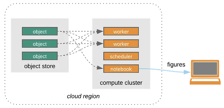
Closed Platforms vs. Open Architectures for Cloud-Native Earth System Analytics

Credit: Open Architecture for scalable cloud-based data analytics. From Abernathey, Ryan (2020): Data Access Modes in Science.
Figure. https://doi.org/10.6084/m9.figshare.11987466.v1
1 2 | # we open the smallest file by size fo_normal = earthaccess.open(ordered[0:1])[0] |
Opening 1 granules, approx size: 0.34 GB
QUEUEING TASKS | : 0%| | 0/1 [00:00<?, ?it/s]
PROCESSING TASKS | : 0%| | 0/1 [00:00<?, ?it/s]
COLLECTING RESULTS | : 0%| | 0/1 [00:00<?, ?it/s]
1 2 3 4 5 6 7 8 9 10 11 | %%time start_time = time.time() ds_normal = xr.open_dataset( fo_normal, group="/gt1l/heights", engine="h5netcdf") t_normal = round(time.time() - start_time, 2) print(f"Opening the data (out-of-region) with xarray took {t_normal} seconds") ds_normal |
Opening the data (out-of-region) with xarray took 953.88 seconds
CPU times: user 19.8 s, sys: 3.6 s, total: 23.4 s
Wall time: 15min 53s
<xarray.Dataset>
Dimensions:         (delta_time: 3376706, ds_surf_type: 5)
Coordinates:
  * delta_time      (delta_time) datetime64[ns] 2022-02-08T03:16:18.010370560...
    lat_ph          (delta_time) float64 ...
    lon_ph          (delta_time) float64 ...
Dimensions without coordinates: ds_surf_type
Data variables:
    dist_ph_across  (delta_time) float32 ...
    dist_ph_along   (delta_time) float32 ...
    h_ph            (delta_time) float32 ...
    pce_mframe_cnt  (delta_time) uint32 ...
    ph_id_channel   (delta_time) uint8 ...
    ph_id_count     (delta_time) uint8 ...
    ph_id_pulse     (delta_time) uint8 ...
    quality_ph      (delta_time) int8 ...
    signal_conf_ph  (delta_time, ds_surf_type) int8 ...
    weight_ph       (delta_time) uint8 ...
Attributes:
    Description:  Contains arrays of the parameters for each received photon.
data_rate: Data are stored at the photon detection rate.3. Let's use the force.

1 2 | earthaccess.login() fo_smart = earthaccess.open(ordered[0:1], smart=True)[0] |
Opening 1 granules, approx size: 0.34 GB
QUEUEING TASKS | : 0%| | 0/1 [00:00<?, ?it/s]
PROCESSING TASKS | : 0%| | 0/1 [00:00<?, ?it/s]
COLLECTING RESULTS | : 0%| | 0/1 [00:00<?, ?it/s]
1 2 3 4 5 6 7 8 9 10 11 12 | %%time start_time = time.time() ds_smart = xr.open_dataset( fo_smart, group="/gt1l/heights", engine="h5netcdf") t_smart = round(time.time() - start_time, 2) print(f"Opening the data (out-of-region) with xarray took {t_smart} seconds with earthacess smart open") ds_smart |
Opening the data (out-of-region) with xarray took 31.42 seconds with earthacess smart open
CPU times: user 1.12 s, sys: 182 ms, total: 1.3 s
Wall time: 31.4 s
<xarray.Dataset>
Dimensions:         (delta_time: 3376706, ds_surf_type: 5)
Coordinates:
  * delta_time      (delta_time) datetime64[ns] 2022-02-08T03:16:18.010370560...
    lat_ph          (delta_time) float64 ...
    lon_ph          (delta_time) float64 ...
Dimensions without coordinates: ds_surf_type
Data variables:
    dist_ph_across  (delta_time) float32 ...
    dist_ph_along   (delta_time) float32 ...
    h_ph            (delta_time) float32 ...
    pce_mframe_cnt  (delta_time) uint32 ...
    ph_id_channel   (delta_time) uint8 ...
    ph_id_count     (delta_time) uint8 ...
    ph_id_pulse     (delta_time) uint8 ...
    quality_ph      (delta_time) int8 ...
    signal_conf_ph  (delta_time, ds_surf_type) int8 ...
    weight_ph       (delta_time) uint8 ...
Attributes:
    Description:  Contains arrays of the parameters for each received photon.
data_rate: Data are stored at the photon detection rate.1 2 3 4 | mean_normal = ds_normal.h_ph.mean() mean_smart = ds_smart.h_ph.mean() assert mean_normal == mean_smart |
1 2 3 4 5 6 7 8 9 10 11 12 | print(f""" 1 data granule Size: {round(ordered[0].size(), 2)} MB Egress: without earthaccess: {round(fo_normal.cache.total_requested_bytes / 1024**2, 2)} MB with earthaccess : {round(fo_smart.cache.total_requested_bytes / 1024**2, 2)} MB Time to science: without earthaccess: {round(t_normal/60, 2)} minutes with earthaccess : {round(t_smart/60, 2)} minutes """) |
1 data granule Size: 349.38 MB Egress: without earthaccess: 3199.29 MB with earthaccess : 112.0 MB Time to science: without earthaccess: 15.9 minutes with earthaccess : 0.52 minutes
5. Why is this important?

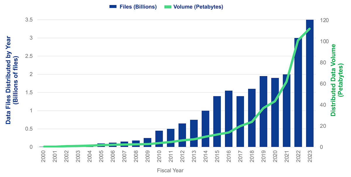
Source: 2023 NASA ESDS Program Highlights
As data in the cloud grows, we need to provide researchers with the means to do cloud native workflows, the simple way!
Cloud native workflows could get expensive, earthaccess can help!
6. Cloud compute with earthaccess, from terabyte to petabyte scale analysis.
We are going to answer a scientific question: "How cold do the Great Lakes get in December?"
Local execution: 10 years, 2 days around Santa's visit. ~ 10GB of HDF
Cloud execution: 20 years, all December. ~ 0.25 TB of HDF
We'll use NASA's GHRSST Level 4 MUR Global Foundation Sea Surface Temperature Analysis (v4.1)
Now you're probably asking, what AWS integration is he going to use? Lambda? Step Functions? Perhaps a novel SQS-powered pipeline...

A Little background story

Me and others talking to Nobel Prize winner Paul Romer, very approchable guy who happens to be a Pythonista. Paris, 2023.
- After talking to Paul Romer, I met some Dask core maintainers and started to chat about our projects. They left NVIDIA to start a company called Coiled.
- They(Coiled) were looking for a simple package to handle NASA APIs for a climate startup, I was looking for ways to unlock the real potential of earthaccess.
- A colaboration from academia and industry led to improvements in earthaccess
1 2 3 4 5 6 7 8 9 10 11 12 13 14 15 16 17 18 19 | %%capture import coiled import dask.bag as db import numpy as np december_ts = [] total_size = 0 total_granules = 0 for year in range(2013, 2023): print(f"Searching for year {year}: ") results = earthaccess.search_data( short_name="MUR-JPL-L4-GLOB-v4.1", # temporal=(f"{year}-12-01", f"{year}-12-31"), temporal=(f"{year}-12-24", f"{year}-12-25"), ) total_size += round(sum([g.size() for g in results]), 2) total_granules += len(results) december_ts.append({f"{year}": results}) |
1 | print(f"granules: {total_granules}, total size: {round(total_size/1024, 2)}GB") |
granules: 20, total size: 9.45GB
“Unfortunately, no one can be told what cloud compute at scale is.
You have to see it for yourself.”
— Luis López

1 2 3 4 5 6 7 8 9 10 11 12 13 14 15 16 17 18 19 20 21 22 23 24 25 26 27 28 29 30 31 32 33 34 35 36 37 38 39 40 41 42 43 44 45 46 47 48 49 50 51 52 | @coiled.function( name="clusty", region="us-west-2", # Run in the same region as data environ=earthaccess.auth_environ(), # Forward Earthdata auth to cloud VMs arm=True, # Use ARM-based instances vm_type="x2gd.medium", local=True ) def process(data): granules, params= data results = [] io_stats = { "total": 0, "hits": 0, "miss": 0 } bbox = params["bbox"] variables = params["variables"] agg = params["agg"] def aggr_func(dataset, op): """Apply different aggregations to an xarray Dataset.""" supported_ops = { 'mean': lambda ds: ds.mean("time"), 'median': lambda ds: ds.median("time"), 'min': lambda ds: ds.min("time"), 'max': lambda ds: ds.max("time"), 'std': lambda ds: ds.std("time")} try: func = supported_ops[op] return func(dataset) except KeyError: raise ValueError(f'"{op}" aggregation operation not supported') earthaccess.login() fileset = earthaccess.open(granules, smart=True) min_lon, min_lat, max_lon, max_lat = bbox for file in fileset: ds = xr.open_dataset(file) ds = ds.sel(lon=slice(min_lon, max_lon), lat=slice(min_lat, max_lat)) # this is particular to this dataset but can be parametrized cond = (ds.sea_ice_fraction < 0.15) | np.isnan(ds.sea_ice_fraction) result = ds.where(cond) results.append(result[variables]) # This is only to keep track of IO io_stats["total"] += file.cache.total_requested_bytes io_stats["hits"] += file.cache.hit_count io_stats["miss"] += file.cache.miss_count cube = xr.concat(results, dim="time") if agg: cube_redux = aggr_func(cube, agg) cube_redux["time"] = cube.time.min().values return (cube_redux, io_stats) return (cube[variables], io_stats) |
Remote code execution, or local code execution... our choice.
1 2 3 4 5 6 7 8 9 10 11 12 | # Step 3: Run function on each file in parallel params = { "bbox" : (-94.93, 40.26, -73.83, 48.95), "variables": ["analysed_sst"], "agg": "mean" } data = list(map(lambda e: (list(e.values())[0], params), december_ts)) dask_bag = db.from_sequence(data) c = dask_bag.map(process) c.visualize() |
1 2 3 4 5 6 7 8 9 10 | %%time computation = process.map(data) dds, iostats = zip(*computation) # This is only to consolidate the i/o stats agg = {key:sum(i[key] for i in iostats if key in i) for key in set(a for l in iostats for a in l.keys())} agg["total"] = agg["total"] / (1024*1024) # MB agg |
CPU times: user 28.9 s, sys: 5.62 s, total: 34.6 s
Wall time: 2min 37s
{'miss': 252, 'hits': 1968, 'total': 1008.0}
1 2 3 4 5 6 7 | ds = xr.concat(dds, dim="time") # transform to celcius ds["analysed_sst"] = ds["analysed_sst"] - 273.15 ds.analysed_sst.attrs['units'] = 'degC' ds |
<xarray.Dataset>
Dimensions:       (time: 10, lat: 870, lon: 2111)
Coordinates:
  * lat           (lat) float32 40.26 40.27 40.28 40.29 ... 48.93 48.94 48.95
  * lon           (lon) float32 -94.93 -94.92 -94.91 ... -73.85 -73.84 -73.83
  * time          (time) datetime64[ns] 2013-12-24T09:00:00 ... 2022-12-24T09...
Data variables:
analysed_sst (time, lat, lon) float32 nan nan nan nan ... nan nan nan nan1 2 3 4 5 6 7 | hvplot.output(widget_location="bottom") ds.analysed_sst.hvplot.contourf( groupby="time", cmap="viridis", x="lon", y="lat", levels=10, coastline=True) |
1 | ds.isel(time=0).sel(lat=[42,44,46,48]).hvplot.kde("analysed_sst", by='lat', alpha=0.5) |
1 | ds.isel(time=3).sel(lat=[42,44,46,48]).hvplot.kde("analysed_sst", by='lat', alpha=0.5) |
1 | print(f"total egress: {round(agg['total']/1024, 2)}gb") |
total egress: 0.98gb
Cloud computing with earthaccess

Thanks to the earthaccess community and the projects that have supported this work!


