Lea Gajdusek | 12112809
Albin Knapp | 12118812
Group project: the Climate System
Instructions
Objectives
In this final project, you will apply the methods you learned over the past weeks to answer the questions below.
Deadline
Please submit your project via OLAT before Thursday January 12 at 00H (in the night from Wednesday to Thursday).
Formal requirements
You will work in groups of two. If we are an odd number of students, one group can have three participants. (Tip: I recommend that students who have not followed my programming class to team up with students who have).
Each group will submit one (executed) jupyter notebook containing the code, plots, and answers to the questions (text in the markdown format). Please also submit an HTML version of the notebook. Each group member must contribute to the notebook. The notebook should be self-contained and the answers must be well structured. The plots must be as understandable as possible (title, units, x and y axis labels, appropriate colors and levels…).
Please be concise in your answer. I expect a few sentences per answer at most - there is no need to write a new text book in this project! Use links and references to the literature or your class slides where appropriate.
Grading
I will give one grade per project, according to the following table (total 10 points):
- correctness of the code and the plots: content, legends, colors, units, etc. (3 points)
- quality of the answers: correctness, preciseness, appropriate use of links and references to literature or external resources (5 points)
- originality and quality of the open research question (2 points)
1 2 3 4 5 6 7 8 9 10 | # Import the tools we are going to need today: import matplotlib.pyplot as plt # plotting library from matplotlib.gridspec import GridSpec import numpy as np # numerical library import xarray as xr # netCDF library import pandas as pd # tabular library import cartopy # Map projections libary import cartopy.crs as ccrs # Projections list # Some defaults: plt.rcParams['figure.figsize'] = (12, 5) # Default plot size |
Part 1 - temperature climatology
Open the ERA5 temperature data:
1 2 | ds = xr.open_dataset('/home/albin/Desktop/programming/WS22-climate/project/data/ERA5_LowRes_Monthly_t2m.nc') #ds = xr.open_dataset(r'C:\Users\leaga\Documents\3SemAW\Climate system\data\ERA5_LowRes_Monthly_t2m.nc') |
Plot three global maps:
- Compute and plot the temporal mean temperature $\overline{T}$ for the entire period (unit °C)
- Compute and plot $\overline{T^{*}}$ (see lesson), the zonal anomaly map of average temperature.
- Compute the monthly average temperature for each month $\overline{T_M}$ (annual cycle). I expect a variable of dimensions (month: 12, latitude: 241, longitude: 480). Hint: remember the
.groupby()command we learned in the lesson. Now plot the average monthly temperature range, i.e. $\overline{T_M}max$ - $\overline{T_M}min$ on a map.
Questions:
- Look at the zonal temperature anomaly map.
- Explain why norther Europe and the North Atlantic region is significantly warmer than the same latitudes in North America or Russia.
- Explain why the Northern Pacific Ocean does not have a similar pattern.
- Look at the average monthly temperature range map.
- Explain why the temperature range is smaller in the tropics than at higher latitudes
- Explain why the temperature range is smaller over oceans than over land
- Where is the temperature range largest? Explain why.
1 2 3 4 5 6 | t2m_tavg = ds.t2m.mean(dim='time') - 273.15 ax = plt.axes(projection=ccrs.Robinson()) t2m_tavg.plot.imshow(ax=ax, transform=ccrs.PlateCarree(), cbar_kwargs={'label': 'Mean temperature [°C]'}) plt.title('Temporal mean temperature (1979-2018)') ax.coastlines(lw=0.5), ax.gridlines(); |

1 2 3 4 5 | t_avg_dep = t2m_tavg - t2m_tavg.mean(dim='longitude') ax = plt.axes(projection=ccrs.Robinson()) t_avg_dep.plot.imshow(ax=ax, transform=ccrs.PlateCarree(), cbar_kwargs={'label': 'Temperature anomaly [°C]'}) plt.title('Zonal anomaly of average temperature 1979 to 2018') ax.coastlines(lw=0.5), ax.gridlines(); |

Q & A
- Explain why norther Europe and the North Atlantic region is significantly warmer than the same latitudes in North America or Russia.
- Because of the thermohaline circulation (Atlantic conveyor belt) -> warm water (a lot of energy) is transported (winds) from the tropics into the north atlantic region, the atmosphere gets warmer and therefore the European climate. North America and Russia don't have such (strong) oceanic circulation, the atmosphere is more influenced by continental weather (e.g. cold air from the poles).
- Explain why the Northern Pacific Ocean does not have a similar pattern.
- "Thermohaline circulation" contains the words "warm" and "salt", which means the circulation is driven by high gradients in temperature and salinity. Like it's seen in the lecture notes (Figure 1.11 from Levitus 1998) both atlantic and pacific ocean have high temp. gradients, but the pacific ocean doesn't have the high salinity the atlantic has (bc of larger freshwater fluxes at the surface) -> stable status where no deep water formation is possible -> no circulation
(Source 1 & 2: lecture notes, lesson 1: Components, characteristic processes, variables and parameters of the climate system)
1 2 3 4 5 6 7 | t2m_mavg = ds.groupby('time.month').mean() t2m_mavg_dif = t2m_mavg.t2m.max(dim='month') - t2m_mavg.t2m.min(dim='month') ax = plt.axes(projection=ccrs.Robinson()) t2m_mavg_dif.plot.imshow(ax=ax, transform=ccrs.PlateCarree(), cmap='Oranges', levels=15, cbar_kwargs={'label': 'Temperature range [°C]'}) plt.title('Average monthly temperature range 1979 to 2018') ax.coastlines(lw=0.5), ax.gridlines(); |

1 | t2m_mavg.sizes |
Frozen({'longitude': 480, 'latitude': 241, 'month': 12})
Q & A
- Explain why the temperature range is smaller in the tropics than at higher latitudes
- In the tropics, the weather is nearly the same all year round, barely changes bc of stable air masses, persistent winds -> no big changes in temperature over the year (more daily cycle due to the changes in cloud cover, rainfall and humidity; short lived, temp. return soon to average). Whereas in higher latitudes there are high seasonal changes due to different solar radiation and the weather (temperature) is influenced by many different weather systems (e.g. fronts) that can occur -> different temperatures possible.
(Source 1)
- Explain why the temperature range is smaller over oceans than over land
- Land has a much lower heat capacity than water -> water can store more of the sun's energy and dispense it later on into the atmosphere (thermal inertia). Whereas over land the temperatures are more volatile, landmasses heat and cool very fast.
- Where is the temperature range largest? Explain why.
- The highest temp. ranges are measured in Siberia/Russia (and also Canada). This is due to the greater distance to the oceans (continental weather). As it has been described in the previous answer, airmasses near oceans have a lower temp. range than airmasses over land.
Part 2 - Precipitation climatology
Open the precipitation file and explore it. The units of monthly precipitation are wrongly labeled (unfortunately). They should read: m per day.
1 2 | ds2 = xr.open_dataset('/home/albin/Desktop/programming/WS22-climate/project/data/ERA5_LowRes_Monthly_tp.nc') #ds2 = xr.open_dataset(r'C:\Users\leaga\Documents\3SemAW\Climate system\data\ERA5_LowRes_Monthly_tp.nc') |
Using .groupby(), compute the average daily precipitation for each month of the year (I expect a variable of dimensions (month: 12, latitude: 241, longitude: 480)). Convert the units to mm per day. Plot a map of average daily precipitation in January and in August with the levels [0.5, 1, 2, 3, 4, 5, 7, 10, 15, 20, 40] and the colormap `YlGnBu'
Questions:
- Describe the location of the ITCZ in January and August. Without going into the details, explain (in one or two sentences)
- Describe the precipitation seasonality in West Africa and in India. Name the phenomenon at play.
1 2 3 4 5 6 7 8 9 10 11 12 13 14 15 16 17 18 19 20 21 22 23 | rain = ds2.groupby('time.month').mean() * 1000 rain_1 = rain.tp.sel(month=1) rain_8 = rain.tp.sel(month=8) plt.figure(figsize = (12,10)) ax = plt.subplot(211, projection=ccrs.Robinson()) rain_1.plot.contourf(ax=ax, levels=[0.5, 1, 2, 3, 4, 5, 7, 10, 15, 20, 40], transform=ccrs.PlateCarree(), cmap='YlGnBu', cbar_kwargs={'label': 'Precipitation [mm/day]'}) plt.title('Average daily precipitation in January') ax.coastlines(lw=0.5), ax.gridlines() ax = plt.subplot(212, projection=ccrs.Robinson()) rain_8.plot.contourf(ax=ax, levels=[0.5, 1, 2, 3, 4, 5, 7, 10, 15, 20, 40], transform=ccrs.PlateCarree(), cmap='YlGnBu', cbar_kwargs={'label': 'Precipitation [mm/day]'}) plt.title('Average daily precipitation in August') ax.coastlines(lw=0.5), ax.gridlines(); |

Q & A
- Describe the location of the ITCZ in January and August. Without going into the details, explain (in one or two sentences)
- In January, the ITCZ is located more southward than in August because of the sun's location. On 21st of December the sun's zenith is located above the southern turning cycle -> more sun energy on southern side of the equator -> ITCZ moves southward. Applies vice versa for the 21st of June, when the sun's zenith is located on the northern turning cycle.
- Describe the precipitation seasonality in West Africa and in India. Name the phenomenon at play.
- This phenomenon is called Monsoon. Bc the ITCZ moves north- and southward within a year, in West Africa and India there are months with very high and very low precipiation (dry and rainy season). In West Africa and India, the rainy season (also called monsoon season) is in JJAS -> bc there the ITCZ is located over these locations for that period. During these months the regions receive about 78% of their total annual precipitation.
Part 3: sea-level pressure and surface winds
Open the file containing the surface winds (u10 and v10) and sea-level pressure (msl).
1 2 | ds3 = xr.open_dataset('/home/albin/Desktop/programming/WS22-climate/project/data/ERA5_LowRes_Monthly_uvslp.nc') #ds3 = xr.open_dataset(r'C:\Users\leaga\Documents\3SemAW\Climate system\data\ERA5_LowRes_Monthly_uvslp.nc') |
Compute $\left[ \overline{SLP} \right]$ (the temporal and zonal average of sea-level pressure). Convert it to hPa, and plot it (line plot). With the help of plt.axhline, add the standard atmosphere pressure line to the plot to emphasize high and low pressure regions. Repeat with $\left[ \overline{u_{10}} \right]$ and $\left[ \overline{v_{10}} \right]$ (in m s$^{-1}$) and add the 0 horizontal line to the plot (to detect surface westerlies from easterlies for example).
Questions:
- Based on your knowledge about the general circulation of the atmosphere, explain the latitude location of the climatological high and low pressure systems of Earth.
- Similarly, explain the direction and strength of the zonal and meridional winds on earth (tip: the sea-level pressure plot helps)
1 2 3 4 5 6 | (ds3.msl.mean(dim=['time', 'longitude']) / 100).plot(label = 'Sea-level pressure $\\left[ \\overline{SLP} \\right]$') plt.axhline(y = 1013.25, label='Standard Atmospheric Pressure', color='r', ls='--') plt.xlim(-90,90) plt.legend(loc='best') plt.ylabel('Pressure [hPa]') plt.title('Sea-level pressure - temporal and zonal average'); |

Q & A
- Based on your knowledge about the general circulation of the atmosphere, explain the latitude location of the climatological high and low pressure systems of Earth.
- climatological high pressure systems
- at about -30°N and 30°N are associated with the subtropical highs where the Hadley cell meets the Ferrell cell on both hemispheres: The warm air risen at the equator sinks in the subtropics, explaining the high pressure systems
- at about -80°N and 80°N correspond to the polar highs: the low temperatures cause the air (cold and dense) to descend, causing high pressure (polar subsidence).
- climatological low pressure systems
- at the Equator (0°N) is due to warm air rising (trade winds from NH and SH converge)
- around -65°N and 60°N: the sub-polar low pressure belts caused by deep lows formed in the extratropics and migrated towards the poleward flank of the extratropical westerlies (Wallace and Hobbs, 2006). Due to less land, the winds - and by extension, the lows - are stronger on the southern subpolar low pressure belt, which can be seen on the plot: pressure down to almost 985 hPa at -65°N vs. ~1012 hPA at 60°N.
1 2 3 4 5 6 7 | ds3.u10.mean(dim=['time', 'longitude']).plot(label = '$\\left[ \\overline{u_{10}} \\right]$ (zonal wind)') ds3.v10.mean(dim=['time', 'longitude']).plot(label = '$\\left[ \\overline{v_{10}} \\right]$ (meridional wind)') plt.axhline(y = 0, color='r', ls='--') plt.xlim(-90,90) plt.ylabel(f'Wind speed [m.s$^-$$^1$]') plt.legend(loc='best') plt.title('Wind directions (zonal, temporal means)'); |

Q & A
- Similarly, explain the direction and strength of the zonal and meridional winds on earth (tip: the sea-level pressure plot helps)
- zonal winds (u-component):
- strong winds in easterly direction (coming from West) centered at -50°N and 50°N: the westerlies ; smaller peaks at -80°N and 80°N: polar easterlies
- strong winds in westerly direction (coming from East) peaks at -15°N and 15°N: respectively the southeast and northeast trade winds ; smaller lows at -85°N, -70°N, 70°N: linked to deviations of the air masses due to the Coriolis effect creating the polar westerlies
- meridional winds (v-component):
- directed to the North: wind speed peaks at -87°N & -70°N (polar easterlies), -10°N (southeast trade winds directed to ITCZ and therefore North), 50°N (northern westerlies)
- directed to the South: -80°N (polar high), -50°N (southern westerlies), 15°N (northeastern trade winds), 70°N (polar easterlies)
- wind directions at ground level: due to cell circulation directions (two neighboring cells i.e. warm/cold air masses of two cells move in opposite direction) ; sudden wind direction changes occur at the boundaries between two atmospheric circulation cells
- wind strength on the SH is greater because winds are faster over flat surfaces (Ocean) than over land (from which there is more on the NH)
(lecture notes, lesson 1: Components, characteristic processes, variables and parameters of the climate system)
Part 4: temperature change and CO$_2$ concentrations
Download the global average CO$_2$ concentration timeseries data in the CSV format (source: NOAA). Here, let me help your read them using pandas:
1 2 | df = pd.read_csv('/home/albin/Desktop/programming/WS22-climate/project/data/co2_mm_gl.csv', skiprows=55, parse_dates={'date' : [0, 1]}, index_col='date') #df = pd.read_csv(r'C:\Users\leaga\Documents\3SemAW\Climate system\data\co2_mm_gl.csv', skiprows=55, parse_dates={'date' : [0, 1]}, index_col='date') |
Prepare three plots:
- plot the monthly global CO$_2$ concentration as a function of time.
- plot the annual average timeseries of global CO$_2$ concentration as a function of time.
- plot the annual average timeseries of global CO$_2$ concentration and of global 2m temperature from ERA5 on the same plot (using a secondary y axis for temperature).
Questions:
- Describe and explain the annual cycle of CO$_2$ concentrations
- What was the CO$_2$ concentration in the atmosphere in the pre-industrial era? Compute the annual increase in CO$_2$ concentration (unit: ppm per year) between 1980 and 1985 and between 2016 and 2021.
- Describe the relationship between global temperatures and CO$_2$ concentrations. Beside CO$_2$, name three processes that can influence temperature variability and change at the global scale.
1 2 3 4 | df.average.plot() plt.title('Monthly global CO$_{2}$ concentrations') plt.ylabel('CO$_{2}$ [ppm]') plt.xlabel('years'); |

1 2 3 4 5 6 | df.average.groupby(df.index.month).mean().plot() plt.title('Averaged monthly global CO$_{2}$ concentration') plt.ylabel('CO$_{2}$ [ppm]') plt.xlabel('months') plt.xlim(1,12) plt.ylim(368,376); |

1 2 3 4 | df.average.groupby(df.index.year).mean().plot() plt.title('Annual global CO$_{2}$ concentration (January 1979 - August 2021)') plt.ylabel('CO$_{2}$ [ppm]') plt.xlabel('years'); |

1 2 3 4 5 6 7 8 | # Meridional weights weight = np.cos(np.deg2rad(ds.latitude)) weight = weight / weight.sum() t2m_weighted = (ds.t2m.mean(dim="longitude") - 273.15) * weight dfc = pd.DataFrame() dfc['temp'] = t2m_weighted.sum(dim="latitude").groupby('time.year').mean(dim="time").to_pandas() ## zonal average !!! dfc['co2'] = df.average.groupby(df.index.year).mean('average') |
1 2 3 4 5 6 7 8 9 | fig, ax1 = plt.subplots() ax1.plot(dfc['temp'], color="blue") ax2 = ax1.twinx() ax2.plot(dfc['co2'], color="darkorange") plt.title('Annual global averages: 2m temperature and CO$_{2}$ concentration') ax1.set_ylabel('temperature [°C]', color='blue') ax2.set_ylabel('CO$_{2}$ [ppm]', color='darkorange'); |

Q & A
- Describe and explain the annual cycle of CO$_2$ concentrations
- rise of CO$_2$ concentration: September until April; decline starting in May (stagnation from April to May on our plot) and minimum reached in September again. Due to unequal land distribution in NH and SH: plants grow in spring and summer, removing CO$_2$ from the atmosphere (decline in CO$_2$ concentration). End of growing season in NH $\longrightarrow$ CO$_2$ builds up again in atmosphere because less land on SH, so unequal amounts of CO$_2$ are removed in the growing seasons of the two hemispheres $\longrightarrow$ annual cycle of CO$_2$ concentration dominated by CO$_2$ concentration cycle on NH (https://site.extension.uga.edu/climate/2015/05/why-is-there-a-seasonal-cycle-in-carbon-dioxide/)
- What was the CO$_2$ concentration in the atmosphere in the pre-industrial era? Compute the annual increase in CO$_2$ concentration (unit: ppm per year) between 1980 and 1985 and between 2016 and 2021.
- 280ppm in the pre-industrial era (https://www.noaa.gov/news-release/carbon-dioxide-now-more-than-50-higher-than-pre-industrial-levels)
1 2 3 | df_increase = df.average.groupby(df.index.year).mean().diff().round(2) print(f'The mean increase in C02 for the years 1980 to 1985 is {df_increase.loc[1980:1985].mean().round(2)} ppm/year.') df_increase.loc[1980:1985] |
The mean increase in C02 for the years 1980 to 1985 is 1.45 ppm/year.
date
1980    2.06
1981    1.20
1982    0.75
1983    1.67
1984    1.54
1985    1.46
Name: average, dtype: float64
1 2 | print(f'The mean increase in C02 for the years 2016 to 2021 is {df_increase.loc[2016:2021].mean().round(2)} ppm/year.') df_increase.loc[2016:2021] |
The mean increase in C02 for the years 2016 to 2021 is 2.51 ppm/year.
date
2016    3.41
2017    2.16
2018    2.39
2019    2.47
2020    2.36
2021    2.27
Name: average, dtype: float64
- Describe the relationship between global temperatures and CO$_2$ concentrations. Beside CO$_2$, name three processes that can influence temperature variability and change at the global scale.
- CO$_2$ is a greenhouse gas $\longrightarrow$ traps infrared radiation emitted by Earth's surface in the Earth's atmosphere $\longrightarrow$ contributes to an increase in global temperatures on average $\longrightarrow$ global temperature rises with CO$_2$ concentrations as seen on the last plot
- processes influencing temperature variability and change at global scale:
- albedo changes
- Milankovitch Cycles (Earth's orbital parameters such as Earth's eccentricity, obliquity, precession)
- volcanism / plate tectonics
Part 5: variability and ENSO (open research question)
Using the available data, describe the global effect of an El Niño year and a La Niña year on sea-surface temperature, precipitation, and air temperature. I suggest to look for literature or a google search on strong ENSO events in the past 40 years, and select one good example for a positive and a negative phase. Then use annual or seasonal anomaly maps to show the patterns of SST, temperature and precipitation anomalies during these events. With citation or links, explain why you picked these years as examples.
Event choice
We chose the 1997/98 El Niño event because it was the first El Niño event to be monitored scientifically from beginning to end (NatGeo) as well as the first to gain attention because of its strength beyond its "usual" impact region (South-East Asia, Australia, South American northern coast) (NOAA: impact on the United States). Even incorporating sea surface temperature uncertainties (see paper on ResearchGate), this event ranks highest (tied with the 2015-16 and 1982-83 El Niño events) on the list of the strongest events. The 1997/98 event caused widespread drought in Australia and Southeast Asia, as well as heavy rainfall and flooding in South America (mainly Peru).
For La Niña, we chose the 2010/11 event (NASA) because the strongest La Niña events mentioned here are not contained in our ERA5 data (which starts in 1979) and neither is the event of 2020/21, which was quite strong, because the ERA5 data covers as last year 2018.
For our comparison/anomaly maps, we chose the month of December as this month usually constitutes the peak of an El Niño/La Niña event.
1 2 | sst = xr.open_dataset('/home/albin/Desktop/programming/WS22-climate/project/data/ERA5_LowRes_Monthly_sst.nc') #sst = xr.open_dataset(r'C:\Users\leaga\Documents\3SemAW\Climate system\data\ERA5_LowRes_Monthly_sst.nc') |
1 2 3 4 5 6 7 8 9 10 11 12 13 14 15 16 17 18 19 20 21 22 23 24 25 26 27 28 29 30 31 32 33 34 35 | sst_12avg = sst.sst.groupby('time.month').mean().sel(month=12) - 273.15 sst_9712 = sst.sst.sel(time='1997-12') - 273.15 sst_1012 = sst.sst.sel(time='2010-12') - 273.15 ## Plot fig = plt.figure(constrained_layout=True, figsize=(12, 9)) gs = GridSpec(2, 2, figure=fig, hspace=0.05, wspace=0.05) ## Mean SST Maps ax = fig.add_subplot(gs[0, :], projection=ccrs.Robinson(central_longitude=200)) sst_12avg.plot.imshow(ax=ax, transform=ccrs.PlateCarree(), levels=[-10, 5, 15, 20, 25, 27.5, 30, 35], cbar_kwargs={'orientation': 'horizontal', 'label': 'mean sea surface temperature [°C]'}) plt.title('mean SST in Decembers from 1979 to 2018') ax.coastlines(lw=0.5), ax.gridlines() ax = fig.add_subplot(gs[1, 0], projection=ccrs.Robinson(central_longitude=200)) sst_9712.plot(ax=ax, transform=ccrs.PlateCarree(), levels=[-10, 5, 15, 20, 25, 27.5, 30, 35], cbar_kwargs={'orientation': 'horizontal', 'label': 'mean sea surface temperature [°C]'}) plt.title('El Niño - mean SST December 1997') ax.coastlines(lw=0.5), ax.gridlines() ax = fig.add_subplot(gs[1, 1], projection=ccrs.Robinson(central_longitude=200)) sst_1012.plot(ax=ax, transform=ccrs.PlateCarree(), levels=[-10, 5, 15, 20, 25, 27.5, 30, 35], cbar_kwargs={'orientation': 'horizontal', 'label': 'mean sea surface temperature [°C]'}) plt.title('La Niña - mean SST December 2010') ax.coastlines(lw=0.5), ax.gridlines() ## Title fig.suptitle('Comparison of SST for strong El Niño and La Niña events', fontsize=20, y=1.05); |

In the plots above, we observe quite a difference of the mean SST for our events: compared to an average year, the mean SST in December 1997 is higher West of Peru and Ecuador whereas the mean SST in December 2020 is unusually lower in the same region compared to the average.
Let's plot these irregularities on anomaly maps and discuss them:
1 2 3 4 5 6 7 8 9 10 11 12 13 14 15 16 17 18 19 20 21 22 23 24 25 26 27 | sst_12avg = sst.sst.groupby('time.month').mean().sel(month=12) sst_ano_9712 = sst.sst.sel(time='1997-12') - sst_12avg sst_ano_1012 = sst.sst.sel(time='2010-12') - sst_12avg fig = plt.figure(figsize=(15, 7)) ## Anomaly SST ax = plt.subplot(121, projection=ccrs.Robinson(central_longitude=200)) sst_ano_9712.plot(ax=ax, transform=ccrs.PlateCarree(), cmap=('bwr'), levels=[-4, -2, -0.5, 0.5, 2, 4], cbar_kwargs={'orientation': 'horizontal', 'label': 'sea surface temperature [°C]'}) plt.title('El Niño - SST anomaly December 1997') ax.coastlines(lw=0.5), ax.gridlines() ax = plt.subplot(122, projection=ccrs.Robinson(central_longitude=200)) sst_ano_1012.plot(ax=ax, transform=ccrs.PlateCarree(), cmap=('bwr'), levels=[-4, -2, -0.5, 0.5, 2, 4], cbar_kwargs={'orientation': 'horizontal', 'label': 'sea surface temperature [°C]'}) plt.title('La Niña - SST anomaly December 2010') ax.coastlines(lw=0.5), ax.gridlines() ## Title fig.suptitle('Anomaly comparison of SST for strong El Niño and La Niña events', fontsize=20, y=0.85); |

The anomaly maps reflect what we saw in the comparison above: warm water during an El Niño event orientated more to the East - towards the west coast of the Americas - than on average.
The unusually high SST in December 1997 (or any other El Niño year) is due to a weakening of the west-blowing trade winds: warm surface water that would otherwise have been blown into the western Pacific builds up in the East and reduces the upwelling of cold water on the coast of South America.
On the opposite, the unusually low SST in December 2010 (or any other La Niña year) is due to an intensifying of the trade winds: more warm surface water is blown into the western Pacific, causing more deepwater upwelling on the coast of South America.
Now let's have a look on the precipitation anomaly map for our selected El Niño and La Niña events:
1 2 3 4 5 6 7 8 9 10 11 12 13 14 15 16 17 18 19 20 21 22 23 24 25 26 27 28 29 30 31 32 33 34 35 36 37 38 39 40 41 42 43 44 45 46 47 48 | pre_12avg = ds2.tp.groupby('time.month').mean().sel(month=12) * 1000 pre_9712 = ds2.tp.sel(time='1997-12') * 1000 pre_1012 = ds2.tp.sel(time='2010-12') * 1000 pre_ano_9712 = pre_9712 - pre_12avg pre_ano_1012 = pre_1012 - pre_12avg plt.figure(figsize=(15, 10)) ## Mean Precipitation Maps ax = plt.subplot(221, projection=ccrs.Robinson(central_longitude=200)) pre_9712.plot(ax=ax, transform=ccrs.PlateCarree(), cmap=('YlGnBu'), levels=[0, 1, 2, 3, 5, 7, 10, 15, 20, 40], cbar_kwargs={'orientation': 'horizontal', 'label': 'precipitation [mm/day]'}) plt.title('El Niño - precipitation December 1997') ax.coastlines(lw=0.5), ax.gridlines() ax = plt.subplot(222, projection=ccrs.Robinson(central_longitude=200)) pre_1012.plot(ax=ax, transform=ccrs.PlateCarree(), cmap=('YlGnBu'), levels=[0, 1, 2, 3, 5, 7, 10, 15, 20, 40], cbar_kwargs={'orientation': 'horizontal', 'label': 'precipitation [mm/day]'}) plt.title('La Niña - precipitation December 2010') ax.coastlines(lw=0.5), ax.gridlines() ## Anomaly Precipitation Maps ax = plt.subplot(223, projection=ccrs.Robinson(central_longitude=200)) pre_ano_9712.plot(ax=ax, transform=ccrs.PlateCarree(), cmap='RdBu', levels = [-15, -10, -6, -2.5, 2.5, 6, 10, 15], cbar_kwargs={'orientation': 'horizontal', 'label': 'precipitation [mm/day]'}) plt.title('El Niño - precipitation anomaly December 1997') ax.coastlines(lw=0.5), ax.gridlines() ax = plt.subplot(224, projection=ccrs.Robinson(central_longitude=200)) pre_ano_1012.plot(ax=ax, transform=ccrs.PlateCarree(), cmap='RdBu', levels = [-15, -10, -6, -2.5, 2.5, 6, 10, 15], cbar_kwargs={'orientation': 'horizontal', 'label': 'precipitation [mm/day]'}) plt.title('La Niña - precipitation anomaly December 2010') ax.coastlines(lw=0.5), ax.gridlines() ## Title plt.suptitle('Comparison of precipitation between 1997/98 El Niño and 2010/11 La Niña', fontsize=20, y=0.95); |

It can be seen that for this 1997/98 El Niño event, the region of high precipitation (ITCZ) in the mid Pacific is located more southwards than normally (as described at NOAA). Furthermore, the widespread droughts on the Southeast Asian islands can be seen, as well as the clearly higher precipitations on the west coast of South America.
The warm water that usually fuels rains (through convection) in the western Pacific stayed in the East. This resulted in cooler ocean temperatures which caused drought in Australia and Indonesia, Malaysia and the Philippines. El Niño weakens also the monsoon
For the 2010/11 La Niña event, our data shows higher precipitations on the Southeast Asian islands and northern coastal Australia. The eastern Pacific off the coast of South America cools (as discussed for the SST plots). The unusually cold ocean cools the atmosphere above it $\longrightarrow$ cool air is dense; doesn’t rise and form storms as easily as warm air $\Longrightarrow$ less rain falls over the cold waters in the eastern equatorial Pacific.
This then caused floodings and mudslides in northern South America and Australia (positive precipitation anomaly on the map), but also widespread drought in Argentina (negative precipitation anomaly).
As we've seen, precipitation and sea surface temperature and closely laced together with the location of the warm water pool determining the convection zones. Now, let's take a look on the influence of the driving events of ENSO on (2m) air temperature:
1 2 3 4 5 6 7 8 9 10 11 12 13 14 15 16 17 18 19 20 21 22 23 24 25 26 27 28 29 30 31 32 33 34 35 36 37 38 39 40 41 42 43 44 45 46 | t2m_12avg = ds.t2m.groupby('time.month').mean().sel(month=12) - 273.15 t2m_9712 = ds.t2m.sel(time='1997-12') - 273.15 t2m_1012 = ds.t2m.sel(time='2010-12') - 273.15 t2m_ano_9712 = (t2m_9712 - t2m_12avg) t2m_ano_1012 = (t2m_1012 - t2m_12avg) plt.figure(figsize=(15, 10)) ## Mean t2m Maps ax = plt.subplot(221, projection=ccrs.Robinson(central_longitude=200)) t2m_9712.plot(ax=ax, transform=ccrs.PlateCarree(), levels = [-10, -5, 0, 5, 10, 15, 20, 23, 26, 28, 30], cbar_kwargs={'orientation': 'horizontal', 'label': 'temperature [°C]'}) plt.title('El Niño - 2m surface temperature December 1997') ax.coastlines(lw=0.5), ax.gridlines() ax = plt.subplot(222, projection=ccrs.Robinson(central_longitude=200)) t2m_1012.plot(ax=ax, transform=ccrs.PlateCarree(), levels = [-10, -5, 0, 5, 10, 15, 20, 23, 26, 28, 30], cbar_kwargs={'orientation': 'horizontal', 'label': 'temperature [°C]'}) plt.title('La Niña - 2m surface temperature December 2010') ax.coastlines(lw=0.5), ax.gridlines() ## Anomaly t2m Maps ax = plt.subplot(223, projection=ccrs.Robinson(central_longitude=200)) t2m_ano_9712.plot(ax=ax, transform=ccrs.PlateCarree(), cmap=('bwr'), levels = [-4, -2.5, -1, 1, 2.5, 4], cbar_kwargs={'orientation': 'horizontal', 'label': 'temperature [°C]'}) plt.title('El Niño - 2m surface temperature anomaly December 1997') ax.coastlines(lw=0.5), ax.gridlines() ax = plt.subplot(224, projection=ccrs.Robinson(central_longitude=200)) t2m_ano_1012.plot(ax=ax, transform=ccrs.PlateCarree(), cmap=('bwr'), levels = [-4, -2.5, -1, 1, 2.5, 4], cbar_kwargs={'orientation': 'horizontal', 'label': 'temperature [°C]'}) plt.title('La Niña - 2m surface temperature anomaly December 2010') ax.coastlines(lw=0.5), ax.gridlines() ## Title plt.suptitle('Comparison of 2m surface temperature between 1997/98 El Niño and 2010/11 La Niña', fontsize=20, y=0.95); |

For both events, the air temperature anomalies coincide with the sea surface temperatures: the ocean water is closely coupled with the air temperature.
We can perfectly observe "The year without winter" (winter 1997/98) in the Midwest of the USA, with knew record-breaking high winter temperatures.
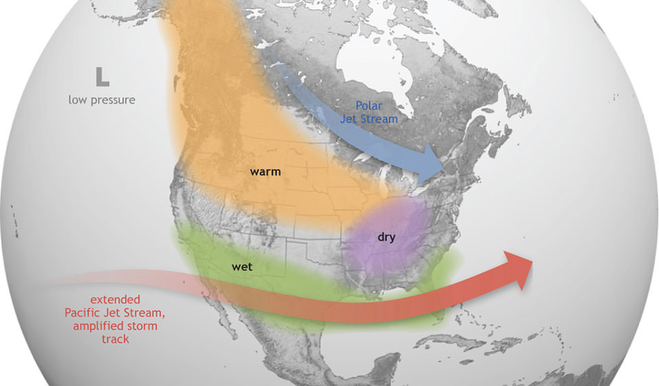
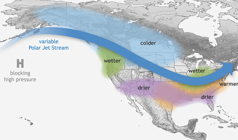
Furthermore we compared our temperature plots with the illustrations from the United States' National Oceanic and Atmospheric Administration NOAA. Similar to the illustration below, our data cleary shows positive temperature anomalies in northern US and western Canada up to Alaska for an El Niño event. In contrast, for a La Niña event we can observe a line of cooler temperatures than the average in the same region, reaching from Alaska across Canada to the east coast, matching the illustrations and patterns from NOAA:
El Niño:
La Niña:
1 |